underworld.function.analytic module
This module provides a suite of models which satisfy the Stokes system of equations.
All models are considered across a unit square (or cube) domain, and utilise (unless otherwise stated) free-slip conditions on all boundaries.
Each model object provides a set of Underworld Functions for description of physical quantities such as velocity, pressure and viscosity.
For numerical validation in Underworld, we construct a Stokes system with appropriate domain and boundary conditions. Viscosity and body forces are set directly using corresponding Function objects provided by the solution class. Generated numerical solution for velocity and pressure (or derived quantities) may then be compared with exact solutions provided by solution objects.
Where appropriate, solution classes provide Latex descriptions of the body force and viscosity functions via the eqn_bodyforce and eqn_viscosity attributes. Note the following definitions for rectangular and step functions:
and
Classes
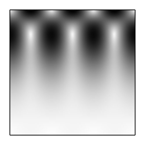
Trigonometric body forcing. |
|
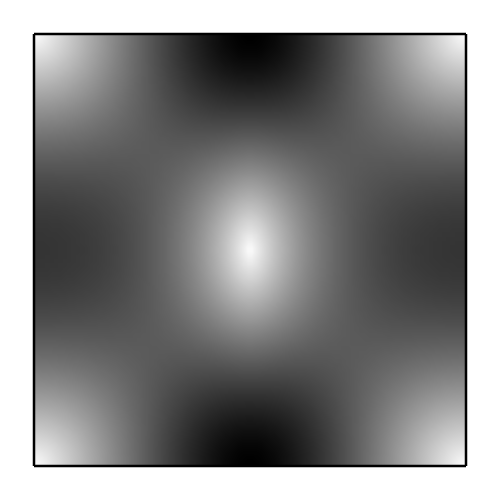
Trigonometric/hyperbolic body forcing. |
|
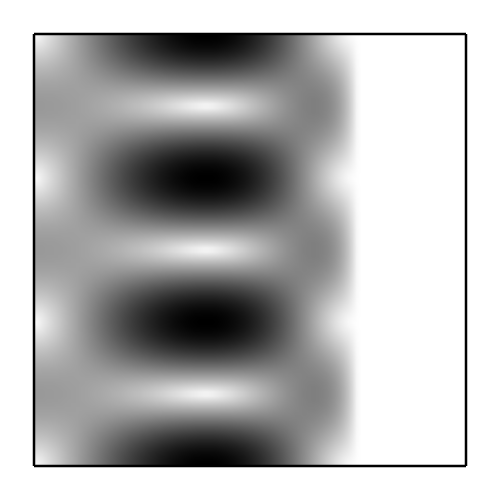
Discontinuous body forcing. |
|
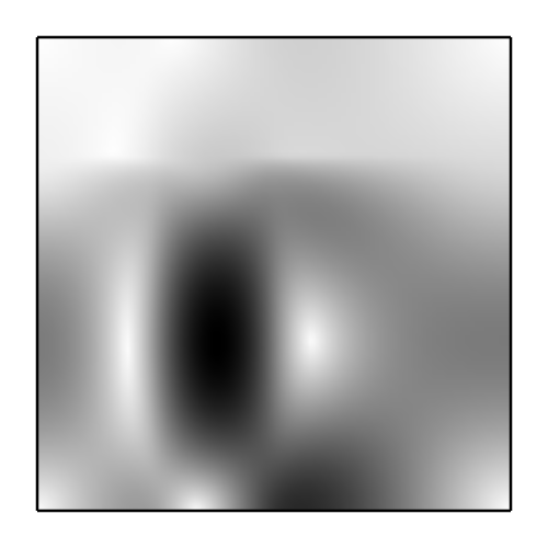
Viscosity step profile in x, trigonometric density profile. |
|
Columnar density profile in x, and viscosity step in z. |
|
This solution uses fixed velocity boundary conditions on all walls along with a constant viscosity. |
|
This solution uses fixed velocity boundary conditions on all walls and a variable viscosity. |
|
Three dimensional solution with density step profile in (x,y). |
|
Trigonometric body forcing. |
|
Trigonometric body forcing. |
|
Sinusoidal viscosity. |
|
Non-linear analytic solution. |
- class underworld.function.analytic.SolA(sigma_0=1.0, n_x=3, n_z=2.0, eta_0=1.0, *args, **kwargs)[source]
Bases:
_SolBaseFreeSlipBcTrigonometric body forcing. Isoviscous.
- Parameters:
sigma_0 (float) – Perturbation strength factor.
n_x (int) – Wavenumber parameter (in x).
n_z (float) – Wavenumber parameter (in z).
eta_0 (float) – Viscosity.
Notes
\[\eta = \eta_0\]\[f = (0,-\sigma_0 \cos(n_x \pi x) \sin(n_z \pi z))\]Viscosity
|Body Force|
|Velocity|
Pressure


- class underworld.function.analytic.SolB(sigma_0=1.0, n_x=3, n_z=2.0, eta_0=1.0, *args, **kwargs)[source]
Bases:
_SolBaseFreeSlipBcTrigonometric/hyperbolic body forcing. Isoviscous.
- Parameters:
sigma_0 (float) – Perturbation strength factor.
n_x (int) – Wavenumber parameter (in x).
n_z (float) – Wavenumber parameter (in z).
eta_0 (float) – Viscosity.
Notes
\[\eta = \eta_0\]\[f = (0,-\sigma_0 \cos(n_x \pi x) \sinh(n_z \pi z))\]Viscosity
|Body Force|
|Velocity|
Pressure


- class underworld.function.analytic.SolC(sigma_0=1.0, x_c=0.5, eta_0=1.0, nmodes=200, *args, **kwargs)[source]
Bases:
_SolBaseFreeSlipBcDiscontinuous body forcing. Isoviscous.
- Parameters:
sigma_0 (float) – Perturbation strength factor.
x_c (float) – Perturbation step location.
eta_0 (float) – Viscosity.
nmodes (int) – Number of Fourier modes used when evaluating analytic solution.
Notes
This solution is quiet slow to evaluate due to large number of Fourier terms required.
Notes
\[\eta = \eta_0\]\[f = (0,-\sigma_0 \operatorname{step}(1,0,x_c; x))\]Viscosity
|Body Force|
|Velocity|
Pressure


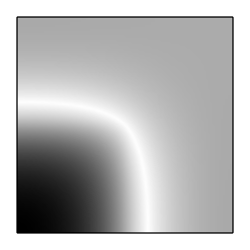
- class underworld.function.analytic.SolCx(n_z=3, eta_A=1.0, eta_B=100000000.0, x_c=0.75, *args, **kwargs)[source]
Bases:
_SolBaseFreeSlipBcViscosity step profile in x, trigonometric density profile.
- Parameters:
n_x (unsigned) – Wavenumber parameter (in x).
eta_A (float) – Viscosity of region A.
eta_B (float) – Viscosity of region B.
eta_c (float) – Viscosity step location.
Notes
\[\eta = \operatorname{step}(\eta_A,\eta_B,x_c; x)\]\[f = (0,-\cos(\pi x) \sin(n_z \pi z))\]Viscosity
|Body Force|
|Velocity|
Pressure


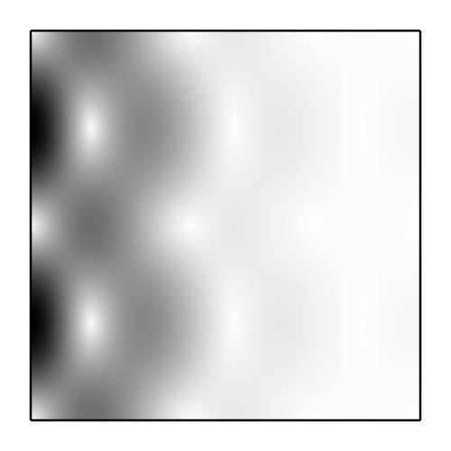
- class underworld.function.analytic.SolDA(sigma_0=1.0, x_c=0.375, x_w=0.25, eta_A=1.0, eta_B=10.0, z_c=0.75, nmodes=200, *args, **kwargs)[source]
Bases:
_SolBaseFreeSlipBcColumnar density profile in x, and viscosity step in z.
- Parameters:
sigma_0 (float) – Perturbation strength factor.
x_c (float) – Centre of column.
x_w (float) – Width of column.
eta_A (float) – Viscosity of region A.
eta_B (float) – Viscosity of region B.
z_c (float) – Viscosity step location.
nmodes (int) – Number of Fourier modes used when evaluating analytic solution.
Notes
\[\eta = \operatorname{step}(\eta_A,\eta_B,z_c; z)\]\[f = (0, -\sigma_0 \operatorname{rect}(x_c,x_w; x) )\]Viscosity
|Body Force|
|Velocity|
Pressure


- class underworld.function.analytic.SolDB2d(*args, **kwargs)[source]
Bases:
_SolBaseFixedBcThis solution uses fixed velocity boundary conditions on all walls along with a constant viscosity. It is originally published in:
Dohrmann, C.R., Bochev, P.B., A stabilized finite element method for the Stokes problem based on polynomial pressure projections, Int. J. Numer. Meth. Fluids 46, 183-201 (2004).
Notes
\[\eta = 1\]Viscosity
|Body Force|
|Velocity|
Pressure


- class underworld.function.analytic.SolDB3d(Beta=4.0, *args, **kwargs)[source]
Bases:
_SolBaseFixedBcThis solution uses fixed velocity boundary conditions on all walls and a variable viscosity. It is originally published in:
Dohrmann, C.R., Bochev, P.B., A stabilized finite element method for the Stokes problem based on polynomial pressure projections, Int. J. Numer. Meth. Fluids 46, 183-201 (2004).
- Parameters:
Beta (float) – Viscosity perturbation strength factor.
Notes
Viscosity
|Body Force|
|Velocity|
Pressure


- class underworld.function.analytic.SolH(sigma_0=1000.0, x_c=0.5, y_c=0.5, eta_0=1.0, nmodes=30, *args, **kwargs)[source]
Bases:
_SolBaseFreeSlipBcThree dimensional solution with density step profile in (x,y). Constant viscosity.
- Parameters:
sigma_0 (float) – Perturbation strength factor.
x_c (float) – Step position (in x).
y_c (float) – Step position (in y).
eta_0 (float) – Viscosity.
nmodes (int) – Number of Fourier modes used when evaluating analytic solution.
Notes
Evaluation of this Fourier based solution is extremely expensive. Default number of mode count is set for fast evaluation, though for high order or high resolution simulations significantly larger mode counts are required. For example, 240 modes are necessary for 64^3 simulations on Q2/dPc1 elements.
Notes
\[\eta = \eta_0\]\[f = (0, 0, -\sigma_0 \operatorname{step}(1, 0, x_c; x) \operatorname{step}(1, 0, y_c; y) )\]Viscosity
|Body Force|
|Velocity|
Pressure


- class underworld.function.analytic.SolKx(sigma_0=1.0, n_x=3, n_z=2.0, B=2.302585092994046, *args, **kwargs)[source]
Bases:
_SolBaseFreeSlipBcTrigonometric body forcing. Exponentially (in x) varying viscosity.
- Parameters:
sigma_0 (float) – Perturbation strength factor.
n_x (int) – Wavenumber parameter (in x).
n_z (float) – Wavenumber parameter (in z).
B (float) – Viscosity parameter.
Notes
\[\eta = \exp(2Bx)\]\[f = (0,-\sigma_0 \cos(n_x \pi x) \sin(n_z \pi z))\]Viscosity
|Body Force|
|Velocity|
Pressure


- class underworld.function.analytic.SolKz(sigma_0=1.0, n_x=3, n_z=2.0, B=2.302585092994046, *args, **kwargs)[source]
Bases:
_SolBaseFreeSlipBcTrigonometric body forcing. Exponentially (in z) varying viscosity.
- Parameters:
sigma_0 (float) – Perturbation strength factor.
n_x (int) – Wavenumber parameter (in x).
n_z (float) – Wavenumber parameter (in z).
B (float) – Viscosity parameter.
Notes
\[\eta = \exp(2Bz)\]\[f = (0,-\sigma_0 \cos(n_x \pi x) \sin(n_z \pi z))\]Viscosity
|Body Force|
|Velocity|
Pressure


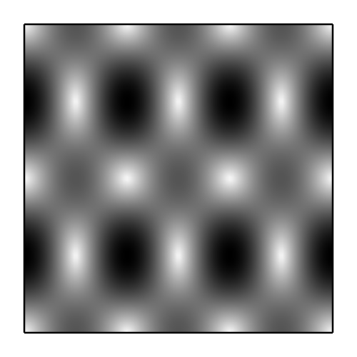
- class underworld.function.analytic.SolM(eta_0=1.0, n_x=3, n_z=2, m_x=4.0, *args, **kwargs)[source]
Bases:
_SolBaseFreeSlipBcSinusoidal viscosity.
- Parameters:
eta_0 (float) – Viscosity perturbation strength factor.
n_x (int) – Velocity wavenumber parameter (in x).
n_z (int) – Velocity wavenumber parameter (in z).
m_x (float) – Viscosity wavenumber parameter (in x).
Notes
\[\eta = 1 + \eta_0(1+\cos(m_x \pi x))\]Viscosity
|Body Force|
|Velocity|
Pressure


- class underworld.function.analytic.SolNL(eta_0=1.0, n_z=1, r=1.5, *args, **kwargs)[source]
Bases:
_SolBaseNon-linear analytic solution. Note that the exactly analytic viscosity (function of position only) is exposed via the standard fn_viscosity attribute, while the non-linear viscosity (function of position and velocity) is exposed via the get_viscosity_nl() method.
- Parameters:
eta_0 (float) – Viscosity perturbation strength factor.
n_z (int) – Velocity wavenumber parameter (in z).
r (float) – Viscosity parameter.
Notes
\[\eta = \eta_0 ( \dot{\eta}_{ij} \dot{\eta}_{ij} )^{(1/r - 1)}\]Viscosity
|Body Force|
|Velocity|
Pressure


- get_bcs(velVar)[source]
( Fixed, Fixed ) conditions vertical walls. ( Free, Fixed ) conditions hortizontal walls.
All fixed DOFs set to analytic soln values.
- Parameters:
velVar (underworld.mesh.MeshVariable) – The velocity variable is required to construct the BC object.
- Returns:
The BC object. It should be passed in to the system being constructed.
- Return type:
- get_viscosity_nl(velocity, pressure)[source]
This method returns a Function object for the non-linear viscosity.
- Parameters:
velocity (underworld.function.Function) – The velocity.
pressure (underworld.function.Function) – The pressure. Pressure is not utilised for this viscosity.