UWGeodynamics User Guide
The Jupyter notebook
The Jupyter notebook provides a powerful environment for the development and analysis of Underworld models. Underworld and UWGeodynamics recommend using Jupyter notebooks for the development of geodynamic models.
If you are not familiar with Jupyter notebooks, we suggest you follow a quick introduction here.
Where to find documentation?
Additional documentation and function specific
documentation can be find in the python doctrings.
You can acces them in the Jupyter notebook by prepending or
appending the method, variable or function with ?.
Design principles

import UWGeodynamics
UWGeodynamics can be imported as follow:
>>> from underworld import UWGeodynamics as GEO
...
Visualization
We provide access to a wrapper around Lavavu , readily available from Underworld.
The visualisation module can be imported as follow
>>> from underworld import visualisation as vis
Warning
Although many plotting modules are available, we strongly encourage people to use the visualisation module. It integrates very well inside the Jupyter notebook, is parallel safe, and can take Underworld function as arguments.
Warning
We provide some basic examples. Look at the Lavavu documentation for more details.
Simple examples:
Plot Material Field or any field / variable defined on the swarm (e.g. plasticstrain, viscosityField, densityField etc.):
>>> from underworld import visualisation as vis
>>> Model = GEO.Model()
>>> Fig = vis.Figure(figsize=(1200,400), title="Material Field")
>>> Fig.Points(Model.swarm, Model.materialField, fn_size=3.0)
...
>>> Fig.show()
>>> Fig.save("MaterialField.png")
'MaterialField.png'
Plot Temperature Field or any field / variable defined on the mesh (e.g. temperature, pressureField, velocityField, strainRateField) as well as projected swarm field / variables (e.g. projMaterialField, projViscosityField etc.)
>>> from underworld import UWGeodynamics as GEO
>>> from underworld import visualisation as vis

>>> u = GEO.u
>>> Model = GEO.Model()
>>> Fig = vis.Figure(figsize=(1200,400), title="Temperature")
>>> Fig.Surface(Model.mesh, GEO.dim(Model.temperature, u.degK))
...
>>> Fig.show()
>>> Fig.save("Temperature.png")
'Temperature.png'
Note
Fields can be dimensionalized using the GEO.dimensionalise function (see below)
Plot Velocity Fields or any vector field.
The example below plots a temperature field with the velocity vectors on top:
>>> from underworld import UWGeodynamics as GEO
>>> from underworld import visualisation as vis

>>> u = GEO.u
>>> Model = GEO.Model()
>>> Fig = vis.Figure(figsize=(1200,400), title="Velocity")
>>> Fig.Surface(Model.mesh, GEO.dim(Model.temperature, u.degK))
...
>>> Fig.VectorArrows(Model.mesh, Model.velocityField)
...
>>> Fig.show()
>>> Fig.save("VelocityField.png")
'VelocityField.png'
Working with units
UWGeodynamics uses Pint, a Python package to define, operate and manipulate physical quantities (A numerical value with unit of measurement). Pint is a very powerful package that handles conversion and operation between units.
We recommend using SI units but other systems are also available.
Pint Unit Registry can be used as follow:
>>> from underworld import UWGeodynamics as GEO
>>> u = GEO.UnitRegistry
or simply
>>> from underworld import UWGeodynamics as GEO
>>> u = GEO.u
You can have a quick overview of all the units available by hitting tab
after the . of the u object.

Quantities can then be defined as follow:
>>> from underworld import UWGeodynamics as GEO
>>> u = GEO.u
>>> length = 100. * u.kilometre
>>> width = 50. * u.kilometre
>>> gravity = 9.81 * u.metre / u.second**2
Pint offers the possibility to append a prefix to the units. 1 million years can thus be defined as follow:
>>> from underworld import UWGeodynamics as GEO
>>> u = GEO.u
>>> length = 1.0 * u.megayear
Note
Unit abbreviation is also possible u.km is equivalent to u.kilometer.
You can refer to the Pint documentation for all abbreviations available.
Model Scaling
Model can be scaled using a series of scaling coefficients
>>> from underworld import UWGeodynamics as GEO
>>> GEO.scaling_coefficients
...
The default scaling coefficients are defined as follow:
Dimension |
value |
|---|---|
[mass] |
1.0 kilogram |
[length] |
1.0 metre |
[temperature] |
1.0 kelvin |
[time] |
1.0 second |
[substance] |
1.0 mole |
The scaling value can be changed by accessing each scaling coefficient as follow
>>> from underworld import UWGeodynamics as GEO
>>> u = GEO.u

>>> GEO.scaling_coefficients["[length]"] = 3. * u.kilometre
>>> GEO.scaling_coefficients["[mass]"] = 4. * u.kilogram
>>> GEO.scaling_coefficients["[temperature]"] = 273.15 * u.degK
>>> GEO.scaling_coefficients["[time]"] = 300. * u.years
The unit entered are checked internally and an error is raised if the units are incompatible. The value is automatically converted to the base units (metre, second, degree, etc).
To scale a model, the user must define a series of characteristic physical values and assign them to the scaling object.
Arguments with units will be scaled by the UWGeodynamics functions.
>>> from underworld import UWGeodynamics as GEO
>>> u = GEO.u

>>> KL = 100 * u.kilometre
>>> Kt = 1. * u.year
>>> KM = 3000. * u.kilogram
>>> KT = 1200. * u.degK

>>> GEO.scaling_coefficients["[length]"] = KL
>>> GEO.scaling_coefficients["[time]"] = Kt
>>> GEO.scaling_coefficients["[mass]"]= KM
>>> GEO.scaling_coefficients["[temperature]"] = KT
dimensionalise / non-dimensionalise
We provide 2 functions GEO.non_dimensionalise and GEO.dimensionalise
to convert between non-dimensional and dimensional values.
The function are also available respectively as GEO.nd and
GEO.dim.
Example:
define a length of 300 kilometres.
use the GEO.nd function to scale it.
convert the value back to SI units.
>>> from underworld import UWGeodynamics as GEO
>>> u = GEO.u

>>> GEO.scaling_coefficients["[length]"] = 300. * u.kilometre

>>> length = 300. * u.kilometre
>>> scaled_length = GEO.nd(length)
>>> print(scaled_length)
1.0
>>> length_metres = GEO.dimensionalise(scaled_length, u.metre)
>>> print(length_metres)
300000.0 meter
The Model object
The central element or “object” of the UWGeodynamics module is the Model object.
It has several uses:
It defines the extent and the outside geometry of your problem.
It works as a container for the field variables.
It basically defines the universe on which you are going to apply physical rules (Gravity field, boundary condition, composition, temperature etc.) It is the equivalent of the box in which you would put the sand and silicon if you were to build an analog experiment in a lab. One important difference is that the “box” his not empty, it is populated with particles that have already some properties. The properties are changed by defining new materials.
>>> from underworld import UWGeodynamics as GEO
>>> u = GEO.u
>>> Model = GEO.Model(elementRes=(64, 64),
...                   minCoord=(0. * u.kilometre, 0. * u.kilometre),
...                   maxCoord=(64. * u.kilometre, 64. * u.kilometre))
The Material object
The UWGeodynamics module is designed around the idea of materials, which are essentially a way to define physical properties across the Model domain.
Predefined Material objects
A library of predefined material is available through the MaterialRegistry object:
from underworld import UWGeodynamics as GEO

materials_database = GEO.MaterialRegistry()
Note
The MaterialRegistry object can import a database of materials from a json file by passing its path as argument. The `default json`__ file can be used as an example.
User defined
Materials are defined using the Material object as follow:
>>> from underworld import UWGeodynamics as GEO

>>> crust = GEO.Material(name="Crust")
Typing the name of the material in an empty cell will return a table which summarizes the property of the material:
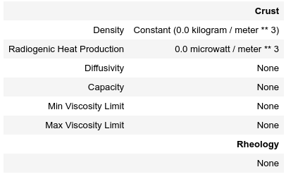
As you can see, most of the property are undefined.
They are several ways to define the physical parametres of our Material.
The first one is to add them directly when creating the object itself:
>>> from underworld import UWGeodynamics as GEO

>>> u = GEO.u
>>> crust = GEO.Material(name="Crust", density=3000*u.kilogram/u.metre**3)
The second option is to change the property after creating the Material:
>>> from underworld import UWGeodynamics as GEO

>>> u = GEO.u
>>> crust = GEO.Material(name="Crust")
>>> crust.density = 3000. * u.kilogram / u.metre **3
The second option is often easier to read.
Warning
UWGeodynamics contains some basic dimensionality checks. Entering wrong units will raise an error
Material can be added to a model as follow:
>>> from underworld import UWGeodynamics as GEO
>>> u = GEO.u
>>> Model = GEO.Model()
>>> crust = Model.add_material(name="Crust")
Although optional, it is a good idea to give a name to the material. The Model.add_material method will return a Material object. That object is a python object that will then be used to define the property of the material.
Material Attributes
The Material object comes with a series of attribute that can be used to define its physical behavior.
Name |
Description |
|---|---|
shape |
Initial Geometrical Representation |
density |
Density |
diffusivity |
Thermal Diffusivity |
capacity |
Thermal Capacity |
radiogenicHeatProd |
Radiogenic Heat Production |
viscosity |
Viscous behavior |
plasticity |
Plastic behavior |
elasticity |
Elastic behavior |
minViscosity |
Minimum Viscosity allowed |
maxViscosity |
Maximum Viscosity allowed |
stressLimiter |
Maximum sustainable stress |
healingRate |
Plastic Strain Healing Rate |
solidus |
Solidus |
liquidus |
Liquidus |
latentHeatFusion |
Latent Heat Fusion (Enthalpy of Fusion) |
meltExpansion |
Melt Expansion |
meltFraction |
Initial Melt Fraction |
meltFractionLimit |
Maximum Fraction of Melt |
viscosityChange |
Change in Viscosity over Melt Fraction range |
viscosityChangeX1 |
Melt Fraction Range begin |
viscosityChangeX2 |
Melt Fraction Range end |
Examples
>>> u = GEO.u
>>> Model = GEO.Model()

>>> Model.density = 200. * u.kg / u.m**3
>>> myMaterial = GEO.Material(name="My Material")
>>> myMaterial.density = 3000 * u.kilogram / u.metre**3
>>> myMaterial.viscosity = 1e19 * u.pascal * u.second
>>> myMaterial.radiogenicHeatProd = 0.7 * u.microwatt / u.metre**3
>>> myMaterial.diffusivity = 1.0e-6 * u.metre**2 / u.second
Global properties
The user can define attributes on the Model itself. The values will be used as global values for materials with undefined attributes
Example
>>> u = GEO.u
>>> Model = GEO.Model()
>>> Model.density = 200. * u.kg / u.m**3
>>> myMaterial = GEO.Material(name="My Material")
The density of myMaterial will default to 200. kilogram / cubic metre unless its density attribute is explicitly specified.
Material shape
The shape attribute essentially describes the initial location of a material. It is used to build the initial geometry of the model.
There are a range of available/pre-defined shapes
Layer (2D/3D)
Polygon (2D)
Box (2D)
Disk (2D)
Spheres (3D)
Annulus (2D)
CombinedShape (Combination of any of the above) (2D)
HalfSpace (3D)
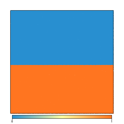
Layer
>>> from underworld import UWGeodynamics as GEO
>>> from underworld import visualisation as vis

>>> u = GEO.u
>>> Model = GEO.Model()
>>> shape = GEO.shapes.Layer(top=30.*u.kilometre, bottom=0.*u.kilometre)
>>> material = Model.add_material(name="Material", shape=shape)

>>> Fig = vis.Figure(figsize=(1200,400))
>>> Fig.Points(Model.swarm, Model.materialField)
...
>>> Fig.show()
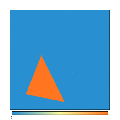
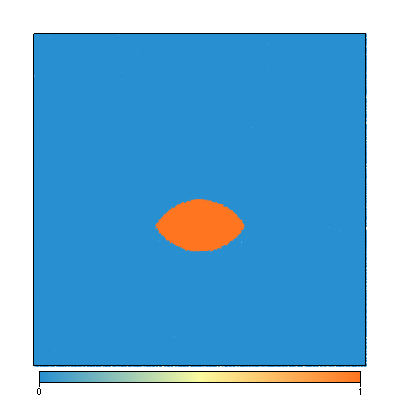
Polygon
>>> from underworld import UWGeodynamics as GEO
>>> from underworld import visualisation as vis

>>> u = GEO.u
>>> Model = GEO.Model()
>>> polygon = GEO.shapes.Polygon(vertices=[(10.* u.kilometre, 10.*u.kilometre),
...                                        (20.* u.kilometre, 35.*u.kilometre),
...                                        (35.* u.kilometre, 5.*u.kilometre)])
>>> material = Model.add_material(name="Material", shape=polygon)

>>> Fig = vis.Figure(figsize=(1200,400))
>>> Fig.Points(Model.swarm, Model.materialField)
>>> Fig.show()
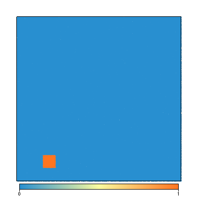
Box
>>> from underworld import UWGeodynamics as GEO
>>> from underworld import visualisation as vis

>>> u = GEO.u
>>> Model = GEO.Model()
>>> box = GEO.shapes.Box(top=10.* u.kilometre, bottom=5*u.kilometre,
...                      minX=10.*u.kilometre, maxX=15*u.kilometre)
>>> material = Model.add_material(name="Material", shape=box)

>>> Fig = vis.Figure(figsize=(1200,400))
>>> Fig.Points(Model.swarm, Model.materialField)
>>> Fig.show()
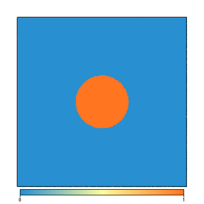
Disk
>>> from underworld import UWGeodynamics as GEO
>>> from underworld import visualisation as vis

>>> u = GEO.u
>>> Model = GEO.Model()
>>> disk = GEO.shapes.Disk(center=(32. * u.kilometre, 32. * u.kilometre),
...                        radius=10.*u.kilometre)
>>> material = Model.add_material(name="Material", shape=disk)

>>> Fig = vis.Figure(figsize=(1200,400))
>>> Fig.Points(Model.swarm, Model.materialField)
>>> Fig.show()
Sphere (3D)
>>> from underworld import UWGeodynamics as GEO

>>> u = GEO.u
>>> Model = GEO.Model(elementRes=(16, 16, 16),
...                   minCoord=(-1. * u.m, -1. * u.m, -50. * u.cm),
...                   maxCoord=(1. * u.m, 1. * u.m, 50. * u.cm))

>>> sphereShape = GEO.shapes.Sphere(center=(0., 0., 20.*u.centimetre),
                                    radius=20. * u.centimetre))
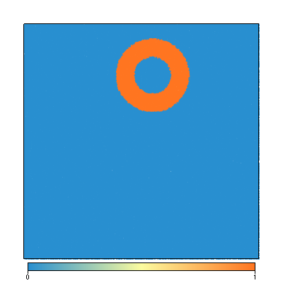
Annulus
>>> from underworld import UWGeodynamics as GEO
>>> from underworld import visualisation as vis

>>> u = GEO.u
>>> Model = GEO.Model()
>>> annulus = GEO.shapes.Annulus(center=(35.*u.kilometre, 50.*u.kilometre),
...                              r1=5.*u.kilometre,
...                              r2=10.*u.kilometre)
>>> material = Model.add_material(name="Material", shape=annulus)

>>> Fig = vis.Figure(figsize=(400,400))
>>> Fig.Points(Model.swarm, Model.materialField)
>>> Fig.show()
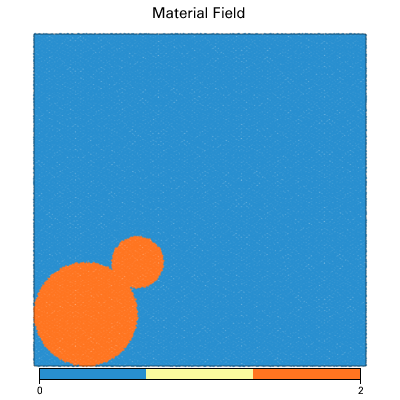
CombinedShape
Several shapes can be combined to form a material shape:
>>> from underworld import UWGeodynamics as GEO
>>> from underworld import visualisation as vis

>>> u = GEO.u
>>> Model = GEO.Model()
>>> disk1 = GEO.shapes.Disk(center=(10. * u.kilometre, 10. * u.kilometre),
...                         radius=10.*u.kilometre)
>>> disk2 = GEO.shapes.Disk(center=(20. * u.kilometre, 20. * u.kilometre),
...                         radius=5.*u.kilometre)

>>> shape = disk1 | disk2
>>> material = Model.add_material(name="Material", shape=shape)

>>> Fig = vis.Figure(figsize=(400,400))
>>> Fig.Points(Model.swarm, Model.materialField)
>>> Fig.show()
You can also take the intersection of some shapes:
>>> from underworld import UWGeodynamics as GEO
>>> from underworld import visualisation as vis

>>> u = GEO.u
>>> Model = GEO.Model()
>>> disk1 = GEO.shapes.Disk(center=(32. * u.kilometre, 32. * u.kilometre),
...                         radius=10.*u.kilometre)
>>> disk2 = GEO.shapes.Disk(center=(32. * u.kilometre, 22. * u.kilometre),
...                         radius=10.*u.kilometre)

>>> shape = disk1 & disk2
>>> material = Model.add_material(name="Material", shape=shape)

>>> Fig = vis.Figure(figsize=(400,400))
>>> Fig.Points(Model.swarm, Model.materialField)
>>> Fig.show()
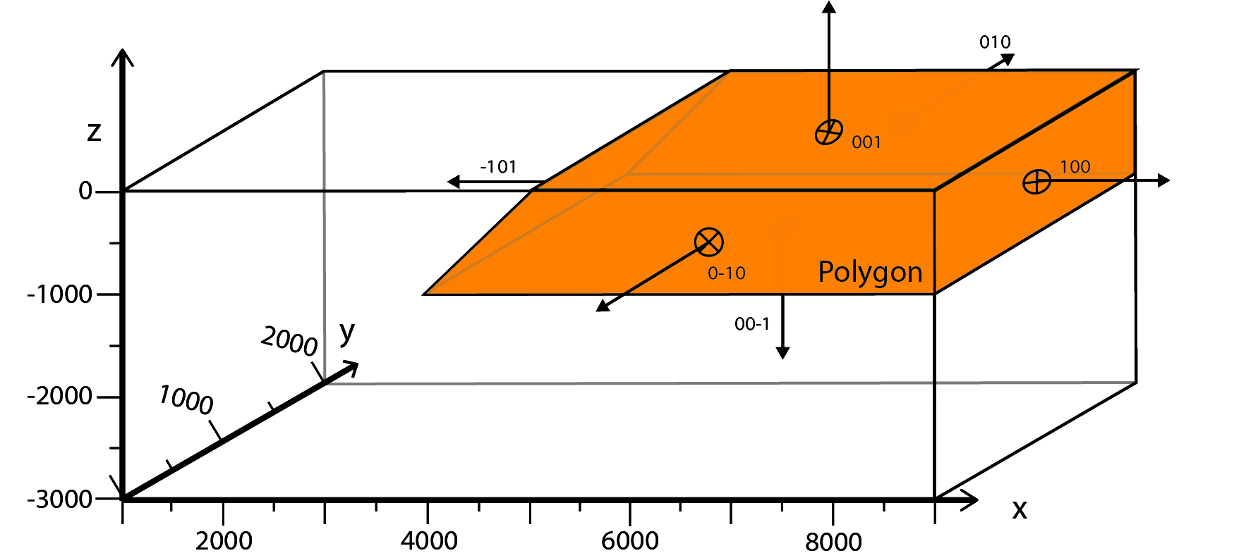
HalfSpace
HalfSpaces can be used to divide space in 2 domains. The divide is a plan defined by its normal vector. The convention is to keep the domain opposite to direction defined by the normal vector.
Note
HalfSpaces can be combined to define 3D shapes / volumes.
>>> from underworld import UWGeodynamics as GEO
>>> from underworld import visualisation as vis
>>> u = GEO.UnitRegistry
>>> Model = GEO.Model(elementRes=(34, 34, 12),
... gravity=(0., 0., -9.81 * u.m / u.s**2),
... minCoord=(0. * u.km, 0. * u.km, -2880. * u.km),
... maxCoord=(9000. * u.km, 2000. * u.km, 20. * u.km))
>>> halfspace1 = GEO.shapes.HalfSpace(normal=(-1.,0.,1.), origin=(4000. * u.km, 0. * u.km, -1000. * u.km))
>>> halfspace2 = GEO.shapes.HalfSpace(normal=(0.,0.,1.), origin=(7000. * u.km, 1000. * u.km, 0. * u.km))
>>> halfspace3 = GEO.shapes.HalfSpace(normal=(1.,0.,0.), origin=(9000. * u.km, 1000. * u.km, -500. * u.km))
>>> halfspace4 = GEO.shapes.HalfSpace(normal=(0.,0.,-1.), origin=(6500. * u.km, 1000. * u.km, -1000. * u.km))
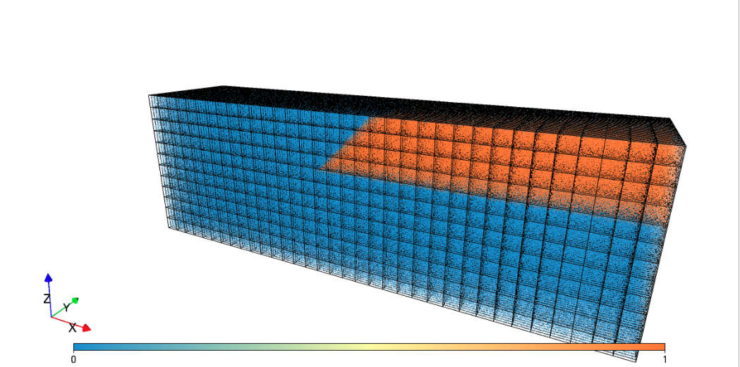
>>> compositeShape = halfspace1 & halfspace2 & halfspace3 & halfspace4
>>> polygon= Model.add_material(name="polygon", shape=compositeShape)
>>> Fig = vis.Figure()
>>> Fig.Points(Model.swarm, Model.materialField, cullface=False, opacity=1.)
>>> Fig.Mesh(Model.mesh)
>>> viewer = Fig.viewer(resolution=(1200,600))
>>> viewer = Fig.viewer(axis=True)
>>> viewer.rotatex(-70)
>>> viewer.rotatey(-10)
>>> viewer.window()
Multiple materials
You can add as many materials as needed:
>>> from underworld import UWGeodynamics as GEO
>>> from underworld import visualisation as vis

>>> u = GEO.u
>>> Model = GEO.Model()

>>> shape = GEO.shapes.Layer(top=30.*u.kilometre, bottom=0.*u.kilometre)
>>> material1 = Model.add_material(name="Material 1", shape=shape)

>>> polygon = GEO.shapes.Polygon(vertices=[(10.* u.kilometre, 10.*u.kilometre),
...                                        (20.* u.kilometre, 35.*u.kilometre),
...                                        (35.* u.kilometre, 5.*u.kilometre)])

>>> material2 = Model.add_material(name="Material 2", shape=polygon)

>>> Fig = vis.Figure(figsize=(400,400))
>>> Fig.Points(Model.swarm, Model.materialField, fn_size=3.)
...
>>> Fig.show()
>>> Fig.save("multiple_materials.png")
'multiple_materials.png'
Temperature and Pressure dependent densities
Temperature and Pressure dependent densities can be assigned to a Material using
the GEO.LinearDensity function which calculates:
where \(\rho\) is the reference density, \(\beta\) a factor, \(\delta P\) the difference between the pressure and the reference pressure, \(\alpha\) is the thermal expansivity and \(\delta T\) is the difference between the temperature and the reference temperature.
>>> from underworld import UWGeodynamics as GEO
>>> u = GEO.u
>>> Model = GEO.Model()

>>> material1 = Model.add_material(name="Material 1", shape=shape)
>>> material1.density = GEO.LinearDensity(reference_density=3370. * u.kilogram / u.metre**3,
...                                       thermalExpansivity= 2.8e-5 * u.kelvin**-1,
...                                       beta=1.0)
Rheologies
Newtonian Rheology
A newtonian rheology can be applied by assigning a viscosity to a already defined material
>>> from underworld import UWGeodynamics as GEO

>>> myMaterial = GEO.Material(name="Newtonian Material")
>>> myMaterial.viscosity = 1e19 * u.pascal * u.second
Non-Newtonian Rheology
Deformation of materials on long timescale is predominantly achieved through viscous diffusion and dislocation creep. Those processes can be expressed using the following equation:
with A the prefactor, \(\dot{\epsilon}\) the square root of the second invariant of the deviatoric strain rate tensor, d the grain size, p the grain size exponent, E the activation energy, P the pressure, V the activation volume, n the stress exponent, R the Gas Constant and T the temperature.
UWGeodynamics provides a library of commonly used Viscous Creep Flow Laws. These can be accessed using the GEO.ViscousCreepRegistry:
Note
The ViscousCreepRegistry object can import a database of rheologies from a json file by passing its path as argument. The `default json`__ file can be find here and can be used as an example.
Example:
>>> from underworld import UWGeodynamics as GEO
>>> material = GEO.Material(name="Material")

>>> rh = GEO.ViscousCreepRegistry()
>>> material.viscosity = rh.Wet_Quartz_Dislocation_Gleason_and_Tullis_1995
You can scale viscosity by using a multiplier. For example to make the Gleason and Tullis, 1995 rheology 30 times stronger you can do:
>>> from underworld import UWGeodynamics as GEO
>>> material = GEO.Material(name="Material")

>>> rh = GEO.ViscousCreepRegistry()
>>> material.viscosity = 30 * rh.Wet_Quartz_Dislocation_Gleason_and_Tullis_1995
The user can of course define their own ViscousCreep rheology.
>>> from underworld import UWGeodynamics as GEO
>>> viscosity = GEO.ViscousCreep(preExponentialFactor=1.0,
...                              stressExponent=1.0,
...                              activationVolume=0.,
...                              activationEnergy=200 * u.kilojoules,
...                              waterFugacity=0.0,
...                              grainSize=0.0,
...                              meltFraction=0.,
...                              grainSizeExponent=0.,
...                              waterFugacityExponent=0.,
...                              meltFractionFactor=0.0,
...                              f=1.0)
Single parametres can then be modified.
viscosity.activationEnergy = 300. * u.kilojoule
Composite Viscosity
Material viscosity can be assigned a combination of viscosities. The effective viscosity is calculated as the harmonic mean of all viscosities.
This is useful to combine diffusion and dislocation creep:
>>> from underworld import UWGeodynamics as GEO

>>> viscosity1 = GEO.ViscousCreep(preExponentialFactor=1.0,
...                              stressExponent=1.0,
...                              activationVolume=0.,
...                              activationEnergy=200 * u.kilojoules,
...                              waterFugacity=0.0,
...                              grainSize=0.0,
...                              meltFraction=0.,
...                              grainSizeExponent=0.,
...                              waterFugacityExponent=0.,
...                              meltFractionFactor=0.0,
...                              f=1.0)


>>> viscosity2 = GEO.ViscousCreep(preExponentialFactor=1.0,
...                              stressExponent=1.0,
...                              activationVolume=0.,
...                              activationEnergy=200 * u.kilojoules,
...                              waterFugacity=0.0,
...                              grainSize=0.0,
...                              meltFraction=0.,
...                              grainSizeExponent=0.,
...                              waterFugacityExponent=0.,
...                              meltFractionFactor=0.0,
...                              f=1.0)
>>> combined_viscosity = GEO.CompositeViscosity([viscosity1, viscosity2])
Plastic Behavior (Yield)
Plastic yielding can be added and will result in rescaling the effective viscosity for a stress limited to the yield stress of the material.
The effective plastic viscosity is given by:
Where \(\dot{\epsilon}\) is the second invariant of the strain rate tensor defined as \(\dot{\epsilon}=\sqrt{\frac{1}{2}\dot{\epsilon}_{ij}\dot{\epsilon}_{ij}}\) The yield value \(\sigma_y\) is defined using a Drucker-Prager yield-criterion:
Setting the friction angle \(\phi=0\) gives the von Mises Criterion. In 2D, equation (2) corresponds to the Mohr-Coulomb criterion, while in 3D it circumscribes the Mohr-Coulomb yield surface.
Linear cohesion and friction weakening can be added by defining their initial and final values over a range of accumulated plastic strain.
As with Viscous Creep, we also provide a registry of commmonly used plastic behaviors. They can be accessed using the GEO.PlasticityRegistry registry.
Note
The PlasticityRegistry object can import a database of plasticity from a json file by passing its path as argument. The `default json`__ file can be find here and can be used as an example.
Users can define their own parametres:
>>> from underworld import UWGeodynamics as GEO
>>> u = GEO.u
>>> Model = GEO.Model()
>>> material = Model.add_material()

>>> material.plasticity = GEO.DruckerPrager(
...     cohesion=10. * u.megapascal,
...     cohesionAfterSoftening=10. * u.megapascal,
...     frictionCoefficient = 0.3,
...     frictionAfterSoftening = 0.2,
...     epsilon1=0.5,
...     epsilon2=1.5)
Viscous Creep and Plastic yielding are combined by assuming that they act in parallel as independent processes. The effective viscoplastic viscosity is calculated as:
Elasticity
Elastic behavior can be added to a material:
>>> from underworld import UWGeodynamics as GEO
>>> u = GEO.u
>>> Model = GEO.Model()
>>> material = Model.add_material()

>>> material.elasticity(shear_modulus=10e9 * u.pascal,
                        observation_time=10000 * u.year)
Simple phase change
One can change the property of one material to another depending on some time, tepmerature, pressure etc. criteria. This is not a phase change sensu-stricto but this allows for simple change such as transition from mantle to oceanic-crust behavior or simply air to water…
Warning
Phase changes can only occur between predefined material. If you plan to add a material during the Model run, you will have to define it beforehand.
In the following example we change air into water when the air particles move below the 0. level.
>>> from underworld import UWGeodynamics as GEO
>>> u = GEO.u
>>> Model = GEO.Model()

>>> air = Model.add_material(name="air")
>>> water = Model.add_material(name="water")
>>> air.phase_changes = GEO.PhaseChange((Model.y < 0.), water.index)
The above example essentially fills the basins with water. For such a specific
purpose you can use the WaterFill class.
>>> air = Model.add_material(name="air")
>>> water = Model.add_material(name="water")
>>> air.phase_changes = GEO.WaterFill(sealevel=0., result=water)
This is easier to read but equivalent.
Melt
Materials can be assigned a Solidus and a Liquidus defined as polynomial
function of temperature. This allows to calculate the fraction of melt present in
the material.
Warning
There is no seggregation of the melt from its source.
A registry of Solidii and Liquidii are available:
>>> from underworld import UWGeodynamics as GEO

>>> solidii = GEO.SolidusRegistry()
>>> crust_solidus = solidii.Crustal_Solidus

>>> liquidii = GEO.LiquidusRegistry()
>>> crust_liquidus = liquidii.Crustal_Liquidus
The percentage of melt results in a linear decrease of the viscosity of a factor
viscosityChange over the viscosityChangeX1 - viscosityChangeX2
melt fraction interval.
The latent heat of fusion is embedded in the energy equation and affects the temperature field of the Model.
The meltExpansion factor affects the density of the materials and equation (1) becomes:
with gamma the factor of melt expansion and F the fraction of melt.
The following example prescribes a decrease in viscosity of 3 order of magnitude over a range of 0.15 to 0.30 fraction of melt. The fraction of the melt is limited to 0.3
>>> from underworld import UWGeodynamics as GEO
>>> u = GEO.u
>>> Model = GEO.Model()

>>> continentalcrust = Model.add_material(name="Continental Crust")
>>> continentalcrust.radiogenicHeatProd = 7.67e-7 * u.watt / u.meter**3
>>> continentalcrust.density  = 2720. * u.kilogram / u.metre**3

>>> continentalcrust.add_melt_modifier(crust_solidus, crust_liquidus,
...                                    latentHeatFusion=250.0 * u.kilojoules / u.kilogram / u.kelvin,
...                                    meltFraction=0.,
...                                    meltFractionLimit=0.3,
...                                    meltExpansion=0.13,
...                                    viscosityChangeX1 = 0.15,
...                                    viscosityChangeX2 = 0.30,
...                                    viscosityChange = 1e-3
...                                   )
...
Mechanical Boundary Conditions
Mechanical boundary conditions are a critical part of any geodynamic model design. In what follows, we quickly detail the options available for defining the mechanical boundary conditions in Underworld using the UWGeodynamics module.
Questions like how to define boundary conditions and to make sure that those are consistent are beyond the scope of this manual.
We will define a simple model for the sake of the example.
>>> from underworld import UWGeodynamics as GEO

>>> u = GEO.u

>>> Model = GEO.Model(elementRes=(64, 64),
...                   minCoord=(0. * u.kilometre, 0. * u.kilometre),
...                   maxCoord=(64. * u.kilometre, 64. * u.kilometre))
Kinematic boundary conditions
Kinematic boundary conditions are set using the set_velocityBCs method. Conditions are defined for each wall (left, right, bottom, top, back and front (3D only)). For each wall, the user must define the condition for each degree of freedom (2 in 2D (x,y), 3 in 3D (x,y,z).
if \(V\) is a vector \((V_x, V_y, V_z)\) that we
want to apply on the left wall, the left parametre must be defined as
left=[Vx, Vy, Vz].
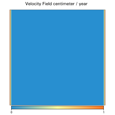
In the following example we set the boundary condition to be:
left wall: \(V_x = -1.0 \text{cm / yr}\), \(Vy = None\)
right wall: \(V_x = 1.0 \text{cm / yr}\), \(Vy=None\)
bottom wall: \(V_x = None\), \(V_y= 0.\) (free slip)
It is an extension model with a total rate of extension equal to 2.0 centimetre / year. No \(V_x\) is prescribed at the bottom, while \(V_y\) is set to \(0.\) no material will be able to enter or leave the model domain from that side. The material is free to move vertically along the side walls.
>>> from underworld import UWGeodynamics as GEO
>>> u = GEO.u
>>> Model = GEO.Model()

>>> Model.set_velocityBCs(left=[1.0*u.centimetre/u.year, None],
...                       right=[-1.0*u.centimetre/u.year, None],
...                       bottom=[None, 0.],
...                       top=[None,0.])
...
3D
Defining boundary conditions for a 3D model is no different than above. The user must define the velocity components with 3 degree of freedom instead of 2.
>>> from underworld import UWGeodynamics as GEO
>>> u = GEO.u
>>> Model = GEO.Model(elementRes=(16, 16, 16),
...                   minCoord=(0. * u.kilometre, 0. * u.kilometre, 0. * u.kilometre),
...                   maxCoord=(64. * u.kilometre, 64. * u.kilometre, 64. * u.kilometre))

>>> Model.set_velocityBCs(left=[1.0*u.centimetre/u.year, None, 0.],
...                        right=[-1.0*u.centimetre/u.year, None, 0.],
...                        bottom=[None, None, 0.],
...                        top=[None, None, 0.],
...                        front=[None, 0., None],
...                        back=[None, 0., None])
...
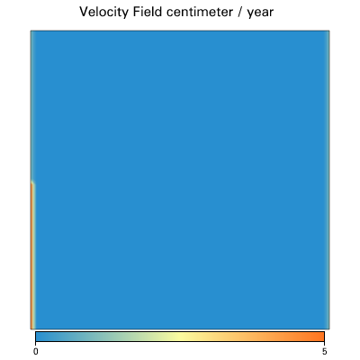
Velocity varying along a wall
At times it is necessary to define a velocity only for a section of a wall and or varying velocities along that wall.
An Underworld function can be passed as a condition.
As an example, we will apply a velocity of \(5.0\text{cm/yr}\) for the part of the left wall below 32 kilometre. Velocity is set to be \(1.0\text{cm/yr}\) above.
>>> from underworld import UWGeodynamics as GEO
>>> u = GEO.u
>>> Model = GEO.Model()

>>> conditions = [(Model.y < GEO.nd(32 * u.kilometre), GEO.nd(5.0 * u.centimetre/u.year)),
                  (True, GEO.nd(1.0*u.centimetre/u.year))]

>>> function = GEO.uw.fn.branching.conditional(conditions)

>>> Model.set_velocityBCs(left=[function, None],
...                       right=[-1.0*u.centimetre/u.year, None],
...                       bottom=[None, 10.*u.megapascal],
...                       top=[None,0.])
...
Stress Conditions
Stress conditions can be applied to the boundaries using the set_stressBCs method:
In the following example we apply a stress of 200.0 megapascal to the bottom of our model:
>>> from underworld import UWGeodynamics as GEO
>>> u = GEO.u
>>> Model = GEO.Model()

>>> Model.set_stressBCs(bottom=[None, 200. * u.megapascal])
...
Note that you will have to make sure that kinematic and stress conditions are compatible.
Frictional Boundaries
Frictional Boundaries can be set as follow:
>>> from underworld import UWGeodynamics as GEO
>>> u = GEO.u
>>> Model = GEO.Model()

>>> Model.set_frictional_boundary(left=frictionCoeff,
...                               right=frictionCoeff,
...                               bottom=frictionCoeff,
...                               top=frictionCoeff,
...                               thickness=3)
...
Where the left, right, top, bottom parametres indicate the side to which you apply a frictional boundary condition on. frictionCoeff is the friction coefficient (tangent of the friction angle in radians). thickness is the thickness of the boundary in number of elements.
Isostasy
Isostasy is an important concept in geodynamics. It is essentially a consequence of the redistribution of mass within a deforming Earth. One important limitation of our geodynamic model is that we model special cases inside rectangular boxes while earth is actually a sphere. One may however need to provide a way to maintain the volume / mass inside the domain in order to mimic isostasy. There is no ideal way to model isostasy in a boxed model, it is however possible to approach isostasy using a support condition.
Options are to:
Balance flows using a kinematic condition at the base of the model.
Balance flows using a stress condition at the base of the model.
Balance flows along the sides.
Lecode Isostasy (kinematic)
The Lecode Isostasy submodule provides a way to model isostatic support at the base of the model. It calculates the velocity to apply at the base of each elemental column. It applies the principles of Airy isostatic model by approximating the weight of each column. The calculation is done dynamically and velocities will change from one step to the next. It is a good option to use in most cases.
The option can be used by creating a LecodeIsostasy object using the
GEO.LecodeIsostasy class. The object requires the index of the
material of reference (the material number). One can apply an average
velocity (calculated across each column base) using the average
parameter (default to False).
>>> from underworld import UWGeodynamics as GEO
>>> u = GEO.u
>>> Model = GEO.Model()

>>> Model.set_velocityBCs(left=[1.0*u.centimetre/u.year, None],
...                       right=[-1.0*u.centimetre/u.year, None],
...                       bottom=[None, GEO.LecodeIsostasy(reference_mat=mantle)],
...                       top=[None,0.])
...
Traction Condition (stress)
Another approach to model isostasy is to defined a certain stress at the base of the model. This is done using units of stress (derived SI units = pascal). The model will then maintain the denfined stress by adjusting the flow across the border/boundary.
>>> from underworld import UWGeodynamics as GEO
>>> u = GEO.u
>>> Model = GEO.Model()

>>> Model.set_stressBCs(bottom=[None, 10.*u.megapascal])
...
Lithostatic Pressure Condition (stress)
The lithostatic pressure field can be passed as a boundary condition (stress)
>>> from underworld import UWGeodynamics as GEO
>>> u = GEO.u
>>> Model = GEO.Model()

>>> Model.set_stressBCs(left=[-Model.lithostatic_pressureField, None])
...
Thermal Boundary Conditions
Absolute temperatures
Setting the temperature at the top of a model to be \(500 \text{kelvin}\) at the top and \(1600 \text{kelvin}\) at the bottom is done as follow.
>>> from underworld import UWGeodynamics as GEO
>>> u = GEO.u
>>> Model = GEO.Model()

>>> Model.set_temperatureBCs(top=500. * u.degK, bottom=1600. * u.degK)
...
You can of course define temperatures on the sidewalls:
>>> from underworld import UWGeodynamics as GEO
>>> u = GEO.u
>>> Model = GEO.Model()

>>> Model.set_temperatureBCs(right=500. * u.degK, left=1600. * u.degK)
...
Fix the temperature of a Material
>>> from underworld import UWGeodynamics as GEO
>>> u = GEO.u
>>> Model = GEO.Model()

>>> Model.set_temperatureBCs(top=500. * u.degK,
...                          bottom=-0.022 * u.milliwatt / u.metre**2,
...                          bottom_material=Model,
...                          materials=[(air, 273. * u.Kelvin)])
...
Note
Model inflow is negative, outflow is positive.
Fix the temperature of internal nodes
You can assign a temperature to a list of nodes by passing a list of node indices (global).
>>> from underworld import UWGeodynamics as GEO
>>> u = GEO.u
>>> Model = GEO.Model()

>>> nodes = [0, 1, 2]
>>> Model.set_temperatureBCs(top=500. * u.degK,
...                          bottom=-0.022 * u.milliwatt / u.metre**2,
...                          bottom_material=Model,
...                          nodeSets=[(273. * u.Kelvin, nodes)])
...
Heat flux
Heat Flux can be assign as follow:
>>> from underworld import UWGeodynamics as GEO

>>> u = GEO.u

>>> Model = GEO.Model()
>>> Material = Model.add_material(shape=GEO.Layer(top=Model.top,
...                                               bottom=Model.bottom)
>>> Model.set_heatFlowBCs(bottom=(-0.22 * u.milliwatt / u.metre**2,
...                               Material))
...
Model initialization
Initialization of the pressure and temperature fields is done by using the
Model.init_model method.
The default behavior is to not initialise the pressure nor the temperature fields.
You can initialise the fields by passing an Underworld function or a Mesh variable. You can initialise the temperature field to steady-state using the “steady-state” value. Yuo can initialise the pressure field to be lithostatic using the “lithostatic” value.
>>> from underworld import UWGeodynamics as GEO
>>> u = GEO.u

>>> Model = GEO.Model()
>>> Model.density = 2000. * u.kilogram / u.metre**3
>>> Model.init_model(temperature="steady-state", pressure="lithostatic")
...
Warning
The lithostatic pressure calculation relies on a regular quadratic mesh. Most of the time this is fine for model initialization as models often starts on a regular mesh. However, this will not work on a deformed mesh
Running the Model
Once your model is set up and initialized. You can run it using the Model.run_for method.
You have 2 options:
Run the model for some given number of steps:
Model.run_for(nstep=10)
Specify an end with duration argument:
Model.run_for(duration=1.0* u.megayears)
which is equivalent to
Model.run_for(1.0*u.megayears)
Specify a timestep
UWGeodynamics calculates the time step automatically based on some numerical stability criteria. You can force a specific time step or force the time step to be constant throughout
Model.run_for(1.0*u.megayears, dt=10000. * u.years)
Saving data
As your model is running you will need to save the results to files.
The Model.run_for method provides a series of arguments to help you save the results at some regular intervals and/or specified times. You can define:
A checkpoint_interval
Model.run_for(endTime=1.0*u.megayears,
              checkpoint_interval=0.1* u.megayears)
The value passed to the checkpoint_interval must have units of time 1. A list of checkpoint times:
Model.run_for(endTime=1.0*u.megayears,
                 checkpoint_interval=0.1* u.megayears,
                 checkpoint_times=[0.85 * u.megayears,
                                   0.21 * u.megayears])
This can be used together or without the checkpoint_interval
UWGeodynamics will save all the fields defined in the
GEO.rcParams[“default.outputs”] list. You can change that list before
running the model.
Checkpointing
By checkpointing we mean saving the data required to restart the Model. This includes the mesh, the swarm and all the associated variables.
However, as the swarm and the swarm variables can be very large and can take a lot of space on disk, the user can decide to save them only every second, third, fourth etc. checkpoint step.
This is done passing the restart_checkpoint argument to the Model.run_for function:
Model.run_for(endTime=1.0*u.megayears,
              checkpoint_interval=0.1* u.megayears,
              restart_checkpoint=2
By default, the swarm and the swarm variables are saved every time the
model reaches a checkpoint time (restart_checkpoint=1).
Pre / Post-solve hook functions
We provide 2 access points for injection of custom functions.
def my_functionA():
    # do something
    print("Hello, I am running a pre-solve function")
    return

def my_functionB():
    # do something
    print("Hello, I am running a post-solve function")
    return

Model.pre_solve_function["A"] = my_functionA
Model.post_solve_function["B"] = my_functionB
Note that the functions are executed in the order they were defined.
Solver Callback functions
User can provide custom callback functions to the solver itself. The function(s) will be executed after each solve. This gives the possibility to tweak the behaviour of the non-linear iterations loop.
def my_function()
    # do something
    print("Hello, This is a solver callback")

Model.callback_function["my_function"] = my_function
Restarting the Model
When checkpointing a model only the mesh, swarms their associates variables are explicitely saved. Since the model state is not explicitly saved, thus the user needs to recreate the Model object before restarting it. In practice, this means the user must run all commands preceding the Model.run_for command.
The user can then restart a model using the restartStep and restartDir arguments:
restartStep is None by default. The step numbercyou want to restart from. If -1, restarts from the last available step in restartDir
restartDir is the folder where the program should look for previously saved data or checkpoints. It is set to Model.outputs by default.
from underworld import UWGeodynamics as GEO

u = GEO.u

Model = GEO.Model(elementRes=(64, 64),
                  minCoord=(0. * u.kilometre, 0. * u.kilometre),
                  maxCoord=(64. * u.kilometre, 64. * u.kilometre))

# Default (restart, restartDir are optional in this case)
Model.run_for(2.0 * u.megayears, restartStep=-1, restartDir="your_restart_directory")

# Restart from step 10
Model.run_for(2.0 * u.megayears, restartStep=10, restartDir="your_restart_directory")

# Overwrite existing outputs
Model.run_for(2.0 * u.megayears, restartStep=False)
Model outputs
All mesh variables / fields defined in the GEO.rcParams["default.outputs"]
are saved as HDF5 files to the outputDir directory at every output times.
An XMF file is provided and can be used to open the files in Paraview
All variables required for a restart are saved as HDF5 files to the
outputDir directory at each checkpoint time.
An XMF file is also provided.
Passive Tracers and tracked fields are also saved as HDF5 files at every output and checkpoint times. Each of then has an associated XMF file.
Parallel run
A Model can be run on multiple processors:
You first need to convert your jupyter notebook to a python script:
jupyter nbconvert --to python my_script.ipynb
You can then run the python script as follow:
mpirun -np 4 python my_script.py
Warning
Underworld and UWGeodynamics functions are parallel safe and can be run on multiple CPUs. This might not be the case with other python libraries you might be interested in using with your Model. For example, matplotlib plots will not work in parallel and must be processed in serial. Tutorial 1 has examples of matplotlib plots which are only done on the rank 0 CPU.
Passive Tracers
>>> from underworld import UWGeodynamics as GEO
>>> import numpy as np

>>> u = GEO.u

>>> Model = GEO.Model()
>>> npoints = 1000
>>> coords = np.ndarray((npoints, 2))
>>> coords[:, 0] = np.linspace(GEO.nd(Model.minCoord[0]), GEO.nd(Model.maxCoord[0]), npoints)
>>> coords[:, 1] = GEO.nd(32. * u.kilometre)
>>> Model.add_passive_tracers(vertices=coords)
You can pass a list of centroids to the Model.add_passive_tracers method. In that case, the coordinates of the passive tracers are relative to the position of the centroids. The pattern is repeated around each centroid.
>>> from underworld import UWGeodynamics as GEO
>>> import numpy as np

>>> u = GEO.u
>>> Model = GEO.Model()
>>> cxpos = np.linspace(GEO.nd(20*u.kilometer), GEO.nd(40*u.kilometer),5)
>>> cypos = np.linspace(GEO.nd(20*u.kilometer), GEO.nd(40*u.kilometer),5)
>>> cxpos, cypos = np.meshgrid(cxpos, cypos)
>>> coords_centroid = np.ndarray((cxpos.size, 2))
>>> coords_centroid[:, 0] = cxpos.ravel()
>>> coords_centroid[:, 1] = cypos.ravel()
>>>
>>> coords = np.zeros((1, 2))
>>> Model.add_passive_tracers(vertices=coords, centroids=coords_centroid)
We provide a function to create circles on a grid:
>>> from underworld import UWGeodynamics as GEO

>>> coords = GEO.circles_grid(radius = 2.0 * u.kilometer,
...                           minCoord=[Model.minCoord[0], lowercrust.bottom],
...                           maxCoord=[Model.maxCoord[0], 0.*u.kilometer])
Tracking Values
Passive tracers can be used to track values of fields at specific location
through time. Tracking projected fields (fields with the prefix proj) is discouraged
as these fields can’t be restarted after checkpointing. Instead, one can track the
non projected field, i.e. projViscosityField, viscosityField)
>>> from underworld import UWGeodynamics as GEO
>>> import numpy as np

>>> u = GEO.u
>>> Model = GEO.Model()

>>> npoints = 1000
>>> coords = np.ndarray((npoints, 2))
>>> coords[:, 0] = np.linspace(GEO.nd(Model.minCoord[0]), GEO.nd(Model.maxCoord[0]), npoints)
>>> coords[:, 1] = GEO.nd(32. * u.kilometre)
>>> Model.add_passive_tracers(name="p1", vertices=coords)

>>> Model.p1_tracers.add_tracked_field(Model.pressureField,
                                       name="tracers_press",
                                       units=u.megapascal,
                                       dataType="float")
>>> Model.p1_tracers.add_tracked_field(Model.strainRateField,
                                       name="tracers_strainRate",
                                       units=1.0/u.second,
                                       dataType="float")
Surface Processes
A range of basic surface processes function are available from the
surfaceProcesses submodule. Surface processes are turned on once you
have passed a valid surface processes function to the
surfaceProcesses method of the Model object.
Example:
>>> from underworld import UWGeodynamics as GEO
>>> u = GEO.u
>>> air = GEO.Material()
>>> sediment = GEO.Material()
>>> Model.surfaceProcesses = GEO.surfaceProcesses.SedimentationThreshold(
...     air=[air], sediment=[sediment], threshold=0. * u.metre)
Three simple function are available:
Total Erosion Above Threshold (
ErosionThreshold).Total Sedimentation Below Threshold (
SedimentationThreshold)Combination of the 2 above. (
ErosionAndSedimentationThreshold)
Erosion and sedimentation rate
Adds an erosion and sedimentation rate to the surface. A pre-defined vertical co-ordinate (surfaceElevation) needs to be defined to stop erodion below that level and sedimenation above it.
Example:
  >>> from underworld import UWGeodynamics as GEO
  >>> u = GEO.u
  >>> air = GEO.Material()
  >>> sediment = GEO.Material()
  >>> Model.surfaceProcesses = GEO.surfaceProcesses.velocitySurface_2D(
  ...     airIndex=air.index, sedimentIndex=sediment.index,
  ...     sedimentationRate= 2.*u.millimeter / u.year, erosionRate= 2.*u.millimeter / u.year,
  ...     surfaceElevation=0.*u.kilometer,
  ...     surfaceArray = coords)

Diffusive surface
~~~~~~~~~~~~~~~~~~~~~~
Adds a linear diffusive surface to the model.

Example:

.. code:: python

   >>> from underworld import UWGeodynamics as GEO
   >>> u = GEO.u
   >>> air = GEO.Material()
   >>> sediment = GEO.Material()
   >>> Model.surfaceProcesses = GEO.surfaceProcesses.diffusiveSurface_2D(
   ...     airIndex=air.index, sedimentIndex=sediment.index,
   ...     D= 1000.0*u.meter**2/u.year,
   ...     surfaceArray = coords)
Coupling with Badlands
UWGeodynamics provides a way to couple an Underworld model to Badlands.
>>> from underworld import UWGeodynamics as GEO
>>> u = GEO.u
>>> air = GEO.Material()
>>> sediment = GEO.Material()
>>> Model.surfaceProcesses = GEO.surfaceProcesses.Badlands(
...     airIndex=[air.index], sedimentIndex=sediment.index,
...     XML="resources/badlands.xml", resolution=1. * u.kilometre,
...     checkpoint_interval=0.01 * u.megayears)
This will allow communication between the UWGeodynamics model and the Badlands surface processes model. Badlands input parameters must be defined inside an XML file as described in the module documentation. We provide an XML example. The resulting Model is a 2-way coupled thermo-mechanical model with surface processes, where the velocity field retrieved from the thermo-mechanical model is used to advect the surface in the Surface Processes Model. The surface in subjected to erosion and deposition. The distribution of materials in the thermomechanical model is then updated.
Users must define a list of material describing the air layers (usually, air and sticky air). It is also require to define an UWGeodynamics.Material object describing the sediment that will be deposited. The index of the Material is passed to the surfaceProcesses function. Users can also provide an Underworld function returning an index of an existing UWGeodynamics.Material.
It is recommended to use a higher spatial resolution in the surface processes model than in the thermo-mechanical model.
Note
When the Thermomechanical model is 2D, the velocity field at the surface is extrapolated in the 3D dimension and the resulting model is a T or 2.5D model (symmetric regional uplift). If the thermomechanical model is 3D the coupling is done in 3D.
Deforming Mesh
Uniaxial deformation can be turned on using the Model.mesh_advector()
method. The method takes an axis argument which defines the direction
of deformation (x=0, y=1, z=2)
>>> Model.mesh_advector(axis=0)
Element are stretched or compressed uniformly across the model. This will result in a change in resolution with time.
Top Free surface
Free surface can be turned on using the Model.freesurface switch.
>>> Model.freesurface = True
Warning
No stabilization algorithm has been implemented yet.
Dynamic rc settings
You can dynamically change the default rc settings in a python script or interactively from the python shell. All of the rc settings are stored in a dictionary-like variable called UWGeodynamics.rcParams, which is global to the UWGeodynamics package. rcParams can be modified directly, for example:
>>> from underworld import UWGeodynamics as GEO
>>> GEO.rcParams['solver'] = "mumps"
>>> GEO.rcParams['penalty'] = 1e6
The UWGeodynamics.rcdefaults command will restore the standard
UWGeodynamics default settings.
There is some degree of validation when setting the values of rcParams,
see UWGeodynamics.rcsetup for details.
Name |
Function |
Default value |
|---|---|---|
CFL |
Set CFL Factor |
0.5 |
solver |
Set Solver |
“mg” (multigrid), options are “mumps”, “lu” |
penalty |
Set penalty value |
0.0 or None |
initial.nonlinear.tolerance |
Set nonlinear tolerance for Stokes first solve |
1e-2 |
nonlinear.tolerance |
Set nonlinear tolerance for solves |
1e-2 |
initial.nonlinear.min.iterations |
Set minimal number of Picard iterations (first solve) |
2 |
initial.nonlinear.max.iterations |
Set maximal number of Picard iterations (first solve) |
500 |
nonlinear.min.iterations |
Set minimal number of Picard iterations |
2 |
nonlinear.max.iterations |
Set maximal number of Picard iterations |
500 |
default.outputs |
List of fields to be saved at checkpoint |
[“temperature”, “pressureField”, “strainRateField”, “velocityField”, “projStressField”, “projTimeField”, “projMaterialField”, “projViscosityField”, “projPlasticStrain”, “projDensityField”] |
swarm.particles.per.cell.2D |
Initial number of particles per cell for 2D models |
40 |
swarm.particles.per.cell.3D |
Initial number of particles per cell for 3D models |
120 |
popcontrol.particles.per.cell.2D |
Minimum number of particles per cell |
40 |
popcontrol.particles.per.cell.3D |
Maximum number of particles per cell |
120 |
popcontrol.aggressive |
Turn on Aggressive population control |
True |
popcontrol.split.threshold |
Population control split threshold |
0.15 |
popcontrol.max.splits |
Population control maximum number of splits |
10 |
shear.heating |
Turn shear heating on / off |
False |
surface.pressure.normalization |
Turn surface pressure normalization on / off |
True |
pressure.smoothing |
Turn pressure smoothing after solve on / off |
True |
advection.diffusion.method |
Advection Diffusion solve method |
“SUPG” |
rheologies.combine.method |
Visco-plastic rheology combination |
“Minimum”, options are “Minimum”, “Harmonic” |
averaging.method |
Multi-material element averaging method |
“arithmetic” options are “arithmetic”, “geometric”, “harmonic”, “maximum”, “minimum”, “root mean square” |
time.SIunits |
Default output units for time field |
u.year |
viscosityField.SIunits |
Default output units for viscosity field |
u.pascal * u.second |
densityField.SIunits |
Default output units for density field |
u.kilogram / u.metre**3 |
velocityField.SIunits |
Default output units for velocity field |
u.centimetre / u.year |
temperature.SIunits |
Default output units for temperature field |
u.degK |
pressureField.SIunits |
Default output units for pressure field |
u.pascal |
strainRateFieldSIunits |
Default output units for strain rate field |
u.pascal |
projStressTensor.SIunits |
Default output units for mesh projected stress tensor field |
u.pascal |
projStressField.SIunits |
Default output units for mesh projected stress field |
u.pascal |
projViscosityFIeld.SIunits |
Default output units for mesh projected viscosities |
u.pascal * u.second |
projTimeField.SIunits |
Default output units for mesh projected time field. |
u.year |
The uwgeodynamicsrc file
UWGeodynamics uses uwgeodynamicsrc configuration files to customize
all kinds of properties, which we call rc settings or
rc parameters. For now, you can control the defaults of a limited
set of properties.
UWGeodynamics looks for uwgeodynamicsrc in four locations, in the following order:
uwgeodynamicsrcin the current working directory, usually used for specific customizations for a particular model setup that you do not want to apply elsewhere.$UWGEODYNAMICSRCif it is a file, else$UWGEODYNAMICSRC/uwgeodynamicsrc.It next looks in a user-specific place, depending on your platform:
On Linux, it looks in
.config/uwgeodynamics/uwgeodynamicsrc(or$XDG_CONFIG_HOME/uwgeodynamics/uwgeodynamicsrc) if you’ve customized your environment.On other platforms, it looks in
.uwgeodynamics/uwgeodynamicsrc.
{INSTALL}/UWGeodynamics/uwgeo-data/uwgeodynamicsrc, where{INSTALL}is something like/usr/lib/python2.7/site-packageson Linux, and maybeC:\\Python27\\Lib\\site-packageson Windows. Every time you install UWgeodynamics, this file will be overwritten, so if you want your customizations to be saved, please move this file to your user-specific directory.
To display where the currently active uwgeodynamicsrc file was
loaded from, one can do the following:
>>> from underworld import UWGeodynamics as GEO
>>> GEO.uwgeodynamics_fname()
'/workspace/user_data/UWGeodynamics/UWGeodynamics/uwgeo-data/uwgeodynamicsrc'
See below for a sample.